Who Said Neural Networks Aren't Linear?
-
ArXiv URL: http://arxiv.org/abs/2510.08570v1
-
Authors: Assaf Hallak; Nimrod Berman; Assaf Shocher
-
Publishing Institutions: Ben-Gurion University; NVIDIA; Technion
TL;DR
This paper proposes a new architecture called Linearizer. By placing a linear operator between two invertible neural networks, it makes traditional nonlinear mappings behave as strict linear transformations in a specially constructed vector space, thereby enabling powerful tools from linear algebra, such as SVD and the pseudoinverse, to be applied to deep learning models.
Key Definitions
The core idea of this paper is to redefine the vector space so that nonlinear functions become linear on it. The key definitions are as follows:
-
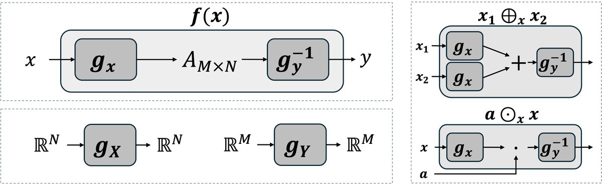
Linearizer: A composite-function architecture of the form $f(x) = \mathbb{L}_{{g_x, g_y, A}}(x) = g_y^{-1}(A g_x(x))$. Here, $g_x$ and $g_y$ are invertible neural networks, and $A$ is a linear operator (matrix). This architecture is nonlinear in the standard Euclidean space.
- Induced Vector Space Operations: New vector addition and scalar multiplication defined based on an invertible network $g$. For vectors $v_1, v_2$ and scalar $a$, the operations are defined as:
- Vector addition: $v_1 \oplus_g v_2 := g^{-1}(g(v_1) + g(v_2))$
- Scalar multiplication: $a \odot_g v_1 := g^{-1}(a \cdot g(v_1))$ With these operations, the set $\mathbb{R}^N$ and the scalar field $\mathbb{R}$ form a new vector space $(V, \oplus_g, \odot_g)$.
-
Induced Inner Product: A new inner product defined in the same way based on an invertible network $g$, making the induced vector space a Hilbert space. It is defined as:
\[\langle v_1, v_2 \rangle_g := \langle g(v_1), g(v_2) \rangle_{\mathbb{R}^N}\]
where the right-hand side is the standard Euclidean inner product.
Related Work
Current neural network models are well-known nonlinear models. While this gives them strong expressive power, it also prevents them from leveraging the rich and elegant theoretical tools of classical linear algebra. In linear systems, operations such as eigendecomposition, inversion, and projection have clear structure and theoretical guarantees, and iterating a linear operator also simplifies the problem. But in nonlinear systems, these tasks become extremely complex, usually requiring specially designed loss functions and optimization strategies, and the results are often only approximate.
The core question this paper aims to address is: can we reinterpret a nonlinear model as a linear operator without sacrificing its expressive power? If so, then we could directly use the full toolkit of linear algebra to analyze and manipulate these complex nonlinear models.
Method
Architecture
The core method proposed in this paper is the Linearizer architecture. Its structure places a linear operator (matrix $A$) between two invertible neural networks $g_x$ and $g_y$:
\[f(x) = g_y^{-1}(A g_x(x))\]Here, $g_x$ maps the input data $x$ into a latent space, $A$ performs a linear transformation in that latent space, and then $g_y^{-1}$ maps the result back to the output space.
Innovations
The essential innovation of Linearizer is that it proves the function $f$ is strictly linear in the new vector space induced by $g_x$ and $g_y$. Specifically:
-
Constructive Linearization: By defining new addition $\oplus$ and scalar multiplication $\odot$ operations, the paper constructs new vector spaces for the input and output. The input space $\mathcal{X}$ is defined by $(\oplus_x, \odot_x)$ (based on $g_x$), and the output space $\mathcal{Y}$ is defined by $(\oplus_y, \odot_y)$ (based on $g_y$). Under this framework, the function $f$ satisfies the superposition principle, i.e., it is proven to be linear:
\[f(a_1 \odot_x x_1 \oplus_x a_2 \odot_x x_2) = a_1 \odot_y f(x_1) \oplus_y a_2 \odot_y f(x_2)\] -
Geometric Intuition: The invertible mapping $g_x$ can be viewed as a diffeomorphism that “straightens” the curved manifold in data space into a flat space in latent space. Therefore, transformation paths that are complex in data space become simple straight lines in latent space.
Advantages
This linearized construction endows the model with a series of powerful algebraic properties, which can be realized directly by operating on the core matrix $A$:
- Composition: The composition of two Linearizers that share the intermediate invertible network $g_y$ is still a Linearizer, and its core matrix is the product of the two original matrices $A_2 A_1$.
-
Iteration: When $g_x = g_y = g$, applying $f$ N times is equivalent to raising matrix $A$ to the Nth power:
\[f^{\circ N}(x) = g^{-1}(A^N g(x))\] -
Transpose: The transpose $f^\top$ of function $f$ is also a Linearizer, with core matrix $A^\top$:
\[f^\top(y) = g_x^{-1}(A^\top g_y(y))\] -
Pseudo-inverse: The Moore-Penrose pseudoinverse $f^\dagger$ of function $f$ is likewise a Linearizer, with core matrix given by the pseudoinverse of $A$, namely $A^\dagger$:
\[f^\dagger(y) = g_x^{-1}(A^\dagger g_y(y))\] - Singular Value Decomposition (SVD): The SVD of the entire nonlinear function $f$ can be constructed by performing SVD on the core matrix $A$.
Experimental Conclusions
The paper demonstrates the practical utility of the Linearizer framework through three applications.
One-Step Flow Matching
-
Method: Traditional flow matching (diffusion) models require multi-step iterative integration to generate data from noise, which is slow. This paper builds the flow matching model as a Linearizer architecture. In the induced linear space, the multi-step Euler integration $\prod_{i=0}^{N-1}(I+\Delta t\,A_{t_i})$ can be collapsed into a single matrix $B$. As a result, the generation process is simplified from a multi-step iterative procedure to a single forward pass:
\[\hat{x}_1 = g^{-1}(B g(x_0))\] -
Conclusion:
- One-step generation: On the MNIST and CelebA datasets, the method achieves high-quality one-step generation, with outputs visually indistinguishable from 100-step iterative generation (MSE of $3.0 \times 10^{-4}$).
- Performance validation: The FID score of one-step generation is comparable to that of 100-step iteration, validating the correctness of the theory.
- Exact inversion: By leveraging the properties of $f^\dagger$, the model can implement an exact encoder, mapping real images back into latent space, something standard diffusion models struggle to do. This makes image reconstruction and interpolation possible.
Quantitative Comparison Results
| Dataset | Inversion-Reconstruction Consistency (LPIPS) | 100-step vs 1-step Fidelity (LPIPS) |
|---|---|---|
| MNIST | 31.6 / .008 | 32.4 / .006 |
| CelebA | 33.4 / .006 | 32.9 / .007 |
Note: The two values in the table represent LPIPS and PSNR, respectively. Lower LPIPS is better.
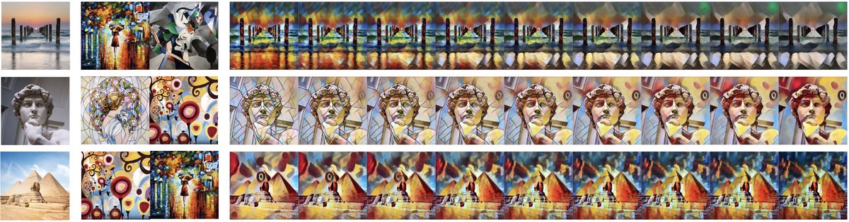
Modular Style Transfer
- Method: Associate different artistic styles with different core matrices $A_{\text{style}}$, while content information is extracted by the shared $g_x$. The style transfer function is $f_{\text{style}}(x) = g_y^{-1}(A_{\text{style}} g_x(x))$.
- Conclusion: This architecture completely separates content and style. Different styles can be easily composed like algebraic objects; for example, smooth transitions between two styles can be achieved by linearly interpolating the two style matrices, $\alpha A_1 + (1-\alpha) A_2$.
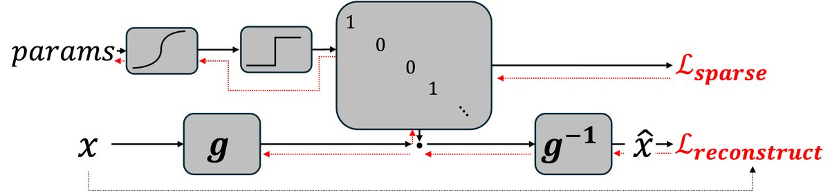
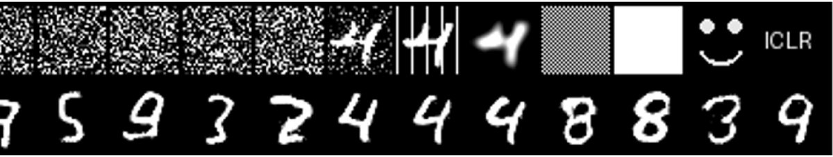
Linear Idempotent Generative Networks
- Method: Idempotence ($f(f(x)) = f(x)$) is very important in both algebra and machine learning. In the Linearizer framework, to make $f$ an idempotent function, it is sufficient to ensure that its core matrix $A$ is idempotent ($A^2=A$), i.e., a projection matrix. This paper directly constructs a differentiable projection matrix through architectural design (using the Straight-Through Estimator), thereby building a generative model that is inherently idempotent.
- Conclusion:
- Global projector: Unlike previous methods that only approximately achieve idempotence near the training data (such as IGNs), the model in this paper is a global projector thanks to its architectural guarantees. It can project any input onto the target data manifold.
- No noise injection required: The model does not inject noise during training, and the entire ambient space can serve as the input source, which is a very unique generative model.