Seesaw: Accelerating Training by Balancing Learning Rate and Batch Size Scheduling

ArXiv URL: http://arxiv.org/abs/2510.14717v1
Authors: Cengiz Pehlevan; Costin-Andrei Oncescu; Depen Morwani; Jingfeng Wu; Alexandru Meterez
Published by: Harvard University; University of California, Berkeley

TL;DR

This paper proposes a training acceleration method called Seesaw, which converts the decay portion of a standard learning rate schedule into an increase in batch size, thereby significantly reducing training wall-clock time by about 36% while maintaining model performance as measured by FLOPs.

Key Definitions

Seesaw: The core scheduling algorithm proposed in this paper. Its principle is that when a standard learning rate scheduler (such as cosine annealing) needs to multiply the learning rate by a factor $\alpha$ ($\alpha < 1$), Seesaw multiplies the learning rate by $\sqrt{\alpha}$ while increasing the batch size by a factor of $1/\alpha$. This transformation is intended to keep the loss dynamics unchanged while reducing the number of serial training steps required by increasing the batch size.
Critical Batch Size (CBS): In training, once the batch size exceeds this value, further increasing the batch size reduces sample efficiency (that is, the model improvement gained per processed sample decreases), thereby limiting gains in training speed. The Seesaw method is mainly effective within the critical batch size.
Normalized SGD (NSGD): A simplified analytical proxy for the Adam optimizer. Its update rule is $\theta_{t} = \theta_{t} - \eta \frac_{t}}{\sqrt{\mathbb{E}\ \mid {\mathbf{g}}_{t}\ \mid ^{2}}}$. This paper uses NSGD to build a theoretical basis for the relationship between learning rate and batch size for adaptive optimizers such as Adam.
Variance-dominated regime: A core assumption in the theoretical analysis of this paper, namely that in the NSGD update rule, the denominator term (the expected squared norm of the gradient, $\mathbb{E}\ \mid {\mathbf{g}}_{t}\ \mid ^{2}$) is determined mainly by the variance of gradient noise rather than the mean of the gradient. This variance term is inversely proportional to batch size, so this assumption usually holds when the batch size does not exceed the critical batch size.

At present, training large language models (LLMs) typically relies on massive computational resources and long training times. A common strategy for reducing wall-clock time is to increase the training batch size to take advantage of data-parallel speedups. However, once the batch size exceeds a “critical batch size” (CBS), simply increasing the batch size harms the model’s convergence efficiency.

Although industry has already been using “batch ramp” strategies (i.e., gradually increasing the learning rate during training) in systems such as LLaMA and OLMo, most of these methods are empirical heuristics and lack a solid theoretical foundation. In particular, for adaptive optimizers such as Adam, the optimal trade-off between learning rate decay and batch size increase remains unclear.

This paper aims to address this issue: to provide a principled, theory-driven framework for batch size scheduling, so that training can be accelerated systematically by increasing batch size rather than relying only on heuristic adjustments.

Method

The core idea of Seesaw is to establish an equivalence between learning rate decay and batch size increase, thereby replacing the original learning rate decay operation with an increase in batch size to reduce the total number of training steps.

Theoretical Derivation from SGD to NSGD

First, the method starts from simple stochastic gradient descent (SGD). Intuitively, for SGD, performing 2 updates with step size $\eta/2$ and batch size $B$ is approximately equivalent (under a first-order Taylor expansion) to performing 1 update with step size $\eta$ and batch size $2B$. This shows that in SGD, the learning rate and batch size roughly follow a linear inverse relationship.

However, for adaptive optimizers like Adam, the relationship is more complex. For theoretical analysis, this paper uses normalized stochastic gradient descent (NSGD) as an analytically tractable proxy for Adam. The update rule of Adam is as follows:

\[\begin{aligned} {\mathbf{m}}_{t} &= \beta_{1}{\mathbf{m}}_{t-1} + (1-\beta_{1}){\mathbf{g}}_{t} \\ {\mathbf{v}}_{t} &= \beta_{2}{\mathbf{v}}_{t-1} + (1-\beta_{2}){\mathbf{g}}_{t}^{2} \\ \theta_{t} &= \theta_{t} - \eta\frac{{\mathbf{m}}_{t}}{\sqrt{{\mathbf{v}}_{t}}+{\epsilon}} \end{aligned}\]

By simplifying the setting (setting $\beta_1=\beta_2=0$ and using a scalar preconditioner), the NSGD update rule can be obtained:

\[\theta_{t} = \theta_{t} - \eta\frac{{\mathbf{g}}_{t}}{\sqrt{\mathbb{E}\ \mid {\mathbf{g}}_{t}\ \mid ^{2}}}\]

Main Contribution

The core innovation of this paper is that, under the “variance-dominated” assumption, it establishes a new learning rate–batch size equivalence relationship for NSGD (and thus Adam).

This assumption states that the denominator $\mathbb{E}\ \mid {\mathbf{g}}_{t}\ \mid ^{2}$ in the update rule is contributed mainly by a variance term that is inversely proportional to batch size, i.e., $\mathbb{E}\ \mid {\mathbf{g}}_{t}\ \mid ^{2} \approx \text{variance} \propto 1/B$. Under this condition, the NSGD update step is approximately $\eta \frac_{t}}{\sqrt{C/B}} \propto (\eta\sqrt{B}) {\mathbf{g}}_{t}$. This shows that the effective learning rate is proportional to $\eta\sqrt{B}$.

To keep the training dynamics unchanged, $\eta\sqrt{B}$ must remain constant. Therefore, if a standard scheduler reduces the learning rate from $\eta$ to $\eta’ = \eta / \alpha_c$, then to find an equivalent batch size $B’$, we need $\eta\sqrt{B} = (\eta/\alpha_c) \sqrt{B’}$, which gives $B’ = B \cdot \alpha_c^2$.

The Seesaw algorithm exploits this relationship: when a standard scheduler (such as cosine annealing) plans to reduce the learning rate by a factor of $\alpha$, Seesaw replaces this operation with:

Reducing the learning rate by a smaller factor of $\sqrt{\alpha}$.
Increasing the batch size by a factor of $\alpha$.

This combination preserves theoretical equivalence ($\text{new learning rate decay factor} \times \sqrt{\text{new batch size increase factor}} = \sqrt{\alpha} \times \sqrt{\alpha} = \alpha = \text{original learning rate decay factor} \times \sqrt{1}$), while reducing the total number of training steps by increasing the batch size.

Seesaw pseudocode: ``$$ Input: η_0 (initial learning rate), B_0 (initial batch size), α > 1 (step decay factor), S (set of steps at which the scheduler reduces η), T (total training steps)

η ← η_0, B ← B_0 for t = 1 to T: if t ∈ S: η ← η / √α; // reduce learning rate B ← B * α; // increase batch size end if // … perform one training step … end for $$``

Advantages

Theory-driven: Unlike heuristic methods, Seesaw is based on an analysis of NSGD dynamics, providing a theoretical foundation for batch scheduling under adaptive optimizers.
Significant acceleration: By converting learning rate decay into batch size increase, Seesaw can reduce wall-clock training time by about 36% (for cosine decay) without sacrificing model performance, approaching the theoretical limit.
Plug-and-play: Seesaw can serve as a direct replacement for existing learning rate schedulers (such as cosine annealing) and is easy to integrate into existing training pipelines.

In addition, the theoretical analysis also derives a stability constraint: $\alpha_{\text{decay}} \geq \sqrt{\beta_{\text{increase}}}$. The strategy adopted by Seesaw, $(\sqrt{\alpha}, \alpha)$, lies exactly on the boundary of this constraint, making it the most aggressive yet stable choice in theory.

Experimental Conclusions

This paper validates the effectiveness of the Seesaw method through experiments on models with 150M, 300M, and 600M parameters. All models were pretrained at Chinchilla scale, i.e., with data size $D=20N$.

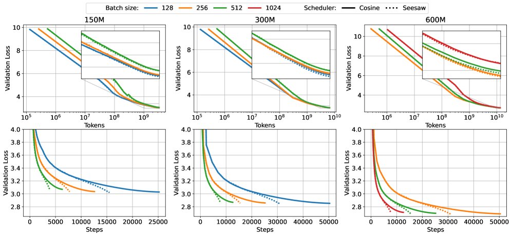The figure above compares Seesaw (orange/green) with standard cosine annealing (blue) across different model scales. The top row (FLOPs vs Loss) shows comparable performance, while the bottom row (Wall Time vs Loss) shows that Seesaw saves significant time.

Summary of key experimental results:

Matched performance, reduced time: Experiments show that within the critical batch size (CBS), Seesaw can match the final validation loss of the standard cosine annealing scheduler (see table below) while reducing wall-clock training time by about 36%. This confirms that Seesaw achieves substantial training acceleration without sacrificing model performance.

Model Size	B=128	B=256	B=512	B=1024
150M (cosine)	3.0282	3.0353	3.0696	3.1214
150M (Seesaw)	3.0208	3.0346	3.0687	3.1318
300M (cosine)	2.8531	2.8591	2.8696	2.9369
300M (Seesaw)	2.8452	2.8561	2.8700	2.9490
600M (cosine)	-	2.6904	2.6988	2.7128
600M (Seesaw)	-	2.6883	2.6944	2.7132

Comparison of final validation loss: Seesaw and cosine annealing perform similarly across different batch sizes.

Verification of theoretical constraints: The experiments validate the most aggressive scheduling strategy derived from theory. As shown in the figure below, when the scheduling strategy violates the stability constraint ($\alpha < \sqrt{\beta}$, as in the red and purple lines), model performance degrades; whereas the boundary strategy used by Seesaw (green line) matches the baseline (blue line) well.

Experiments on the 150M model validate the effectiveness of the theoretical constraint. Overly aggressive batch-increase strategies (red, purple) lead to performance degradation.

Limitations of the method: When the training batch size far exceeds the CBS, Seesaw’s advantage disappears, and its performance can even be worse than standard cosine annealing. As shown below, at very large batch sizes, Seesaw (green) cannot match the baseline (blue). This is because the “variance-dominated” assumption no longer holds in this regime; the noise in the gradients is very small, and learning-rate decay becomes indispensable and can no longer be replaced by increasing batch size.

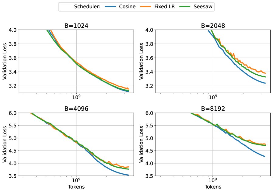At batch sizes far beyond the CBS, Seesaw (green) and other variants cannot match the baseline performance (blue).

Summary

This paper successfully provides a theoretical foundation for batch-size scheduling in LLM training and designs the Seesaw algorithm based on it. Experiments demonstrate that Seesaw is a simple and effective plug-and-play solution that can significantly speed up training without affecting the model’s final performance. Its core contribution is revealing the $\eta \sqrt{B}$ equivalence between learning-rate decay and batch-size increase under adaptive optimizers (under specific conditions), and turning it into a practical acceleration tool. However, the effectiveness of this method is mainly limited to training scenarios within the critical batch size.