Reinforcement learning

ArXiv URL: http://arxiv.org/abs/2405.10369v1
Author: B. Porr; F. Wörgötter
Publishing organization: ASTRON

Introduction

Reinforcement Learning (RL), driven by deep neural networks, has achieved major breakthroughs across multiple disciplines, demonstrating outstanding capabilities in areas such as computer games, board games, robotics, and the development of efficient algorithms for matrix multiplication and sorting.

In astronomy, reinforcement learning has also begun to emerge, with applications including automated telescope control (such as adaptive optics and reflector control), observation scheduling, and hyperparameter tuning in radio astronomy data processing pipelines. Given that modern astronomy can be viewed as an information flow from telescopes to scientists, reinforcement learning is expected to play a greater role in assisting and optimizing many stages of this process, which is also the motivation for this article.

Machine Learning (ML) mainly includes three paradigms:

Supervised learning: Provide the machine with inputs and the corresponding expected outputs so it can learn the task.
Unsupervised learning: Provide the machine with input data only.
Reinforcement learning: The machine learns to perform tasks through repeated trial-and-error interactions with the external environment and by learning from the feedback it receives. Unlike the first two, reinforcement learning has a pronounced temporal dimension, where the task is treated as a sequence of continuous actions rather than a single-step decision.

This article aims to provide a survey of modern deep reinforcement learning, with a focus on its applications in astronomy, offering new users a concise yet comprehensive introductory guide so they can quickly apply the relevant techniques to their own work.

Reinforcement Learning Theory

This section briefly outlines the theoretical foundations of reinforcement learning, mainly from the perspective of machine learning, while also incorporating cross-disciplinary ideas from dynamic programming, cybernetics, and even neuroscience.

States, Actions, and Rewards

The core framework of reinforcement learning involves the interaction between an agent (agent) and its environment (environment), as shown in Figure 1. To achieve a specific goal, the agent performs actions (action) based on observations (observations) received from the environment. After the environment receives an action, its state changes and it feeds back a reward (reward) to the agent, which is a numerical evaluation of the action’s quality.

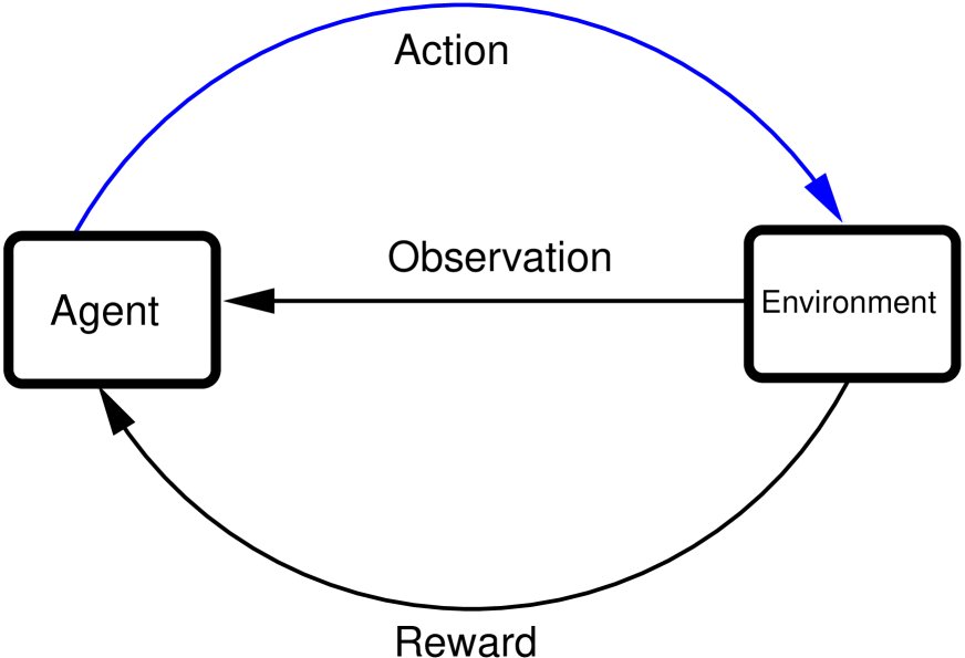
Figure 1: Interaction between the agent and the environment. The agent receives observations, takes actions, and obtains the corresponding rewards.

This interaction process can be described mathematically:

State (State): The set representing the environment state is $\mathcal{S}$, and a single state is denoted by $s$ (usually a vector). A state is a condensed representation of observations.
Action (Action): The set of actions the agent can take is $\mathcal{A}$, and a single action is denoted by $a$ (usually a vector). The state and action spaces can be either discrete or continuous.
Reward (Reward): A scalar value $r$ that measures how good an action is, produced by the reward function $\mathcal{R}$. The principle of reward design is: the more an action helps achieve the final goal, the higher the reward; otherwise, a low reward or a penalty is given.

The table below lists some examples of reinforcement learning applications:

Problem	Goal	State	Action
Chess	Win the game	Positions of all pieces on the board	Select and move a piece
Bipedal robot walking	Walk	Positions, velocities, etc. of leg joints	Apply torque to each leg joint
Self-driving car	Reach the destination	Positions, velocities, accelerations of itself and other vehicles; fuel level, road conditions, road signs, pedestrians, etc.	Apply force to accelerate, brake, steer, etc.

Markov Decision Process

The interaction between the agent and the environment is a continuous loop. At time step $t$, the agent receives state $s_t$ and reward $r_t$, and outputs action $a_t$; after the environment executes $a_t$, it transitions to a new state $s_{t+1}$ and provides a new reward. This process is usually episodic, meaning that after a series of steps it reaches a terminal state (success or failure).

This process can be formalized as a Markov Decision Process (MDP), defined by a quadruple $(\mathcal{S}, \mathcal{A}, \mathcal{R}, \mathcal{P})$. Here $\mathcal{P}$ is the state transition probability. The Markov property means that the state transition probability at time step $t$ depends only on the current state $s_t$ and the action $a_t$ taken, i.e., $p(s_{t+1} \mid s_t, a_t)$.

The learning objective of the agent is not to maximize immediate reward, but to maximize the discounted cumulative reward of future rewards. This introduces the discount factor $\gamma$ ($0 < \gamma < 1$), which balances the importance of short-term and long-term rewards and ensures convergence of the total reward over an infinite time horizon.

Q Function, Value Function, and Policy

To solve RL problems, we introduce several core concepts and illustrate them with a simple maze example (Figure 2). The goal of the agent is to move from any empty cell to the target position in the upper right corner.

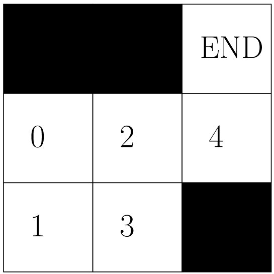
Figure 2: Maze environment, containing 5 valid states (0-4) and 4 actions (up, down, left, right).

To achieve the goal, we define a reward table (Table 2) and introduce a Q table to evaluate the “quality” of each state-action pair.

Table 2: Reward table $R[s, a]$ for the maze environment

State	$\rightarrow$	$\leftarrow$	$\uparrow$	$\downarrow$
0	-1	$-\infty$	$-\infty$	-1
1	-1	$-\infty$	-1	$-\infty$
2	-1	-1	$-\infty$	-1
3	$-\infty$	-1	-1	$-\infty$
4	$-\infty$	-1	100	$-\infty$

By repeatedly iterating and updating the Q table $Q[s,a]$ using Algorithm 1 (a simplified form of Q-learning), we can eventually obtain a converged Q table (Table 3), which guides the agent to choose the optimal action in any state.

Table 3: Converged Q table for the maze environment ($\gamma=0.9$)

State	$\rightarrow$	$\leftarrow$	$\uparrow$	$\downarrow$
0	79.1	0	0	62.171
1	70.19	0	70.19	0
2	89	70.19	0	70.19
3	0	62.171	79.1	0
4	0	0	100	0

For high-dimensional or continuous-space problems, tabular methods are no longer suitable, and function approximators (usually deep neural networks) are needed to represent the following concepts:

Policy: A mapping from states to actions. A deterministic policy $\pi(s)$ directly outputs an action $a$, while a stochastic policy $\pi(a \mid s)$ outputs a probability distribution over actions given a state.
Q-function: The state-action value function $Q(s,a)$, which measures the expected cumulative reward of taking action $a$ in state $s$.
Value function: The state value function $V(s)$, which measures how good it is to be in state $s$, i.e., the expected cumulative reward obtained by following a certain policy starting from that state.

The relationships among these functions are defined by the Bellman equation, which is the foundation of optimality in RL problems:

\[Q(s,a) = r(s,a)+\gamma\underset{a'=\pi(s')}{\mathrm{max}}Q(s',a')\]

Solving an RL problem essentially means learning the optimal policy function $\pi(s)$, Q-function $Q(s,a)$, or value function $V(s)$. Deep neural networks, with their powerful representational capacity and ready-made gradient descent optimization framework, are an ideal choice for representing these functions.

Deep Reinforcement Learning Algorithms

This section focuses on model-free deep reinforcement learning algorithms. When training an intelligent agent, the following challenges are typically encountered:

Insufficient data: Collecting training data through interaction with the environment is costly.
Exploitation vs exploration trade-off: A balance must be struck between exploiting the current best policy and exploring unknown actions to avoid getting stuck in a local optimum. The $\epsilon$-greedy strategy is commonly used, where an action is chosen randomly with probability $\epsilon$ (exploration) and the best action is chosen with probability $1-\epsilon$ (exploitation).
Training instability: The iterative solution process of the Bellman equation can be unstable because the target value to be updated depends on the Q-function itself, which is also being updated.

Experience Replay

To address insufficient data and training instability, experience replay is widely used. This method stores samples from the agent-environment interaction, namely tuples $(s, a, r, s’)$, in a large-capacity storage called a replay buffer $\mathcal{D}$. During training, a mini-batch of data is randomly sampled from $\mathcal{D}$ for learning. This breaks the temporal correlation among data, improves data utilization, and enhances training stability. This training approach, which uses historical data (possibly generated by an old policy), belongs to off-policy algorithms. Algorithm 2 shows the general training procedure using experience replay.

Taxonomy: Algorithms Based on Action Space

This article classifies deep reinforcement learning algorithms according to the type of action space, mainly into discrete-action-space algorithms and continuous-action-space algorithms.

Reinforcement Learning in Discrete Action Spaces

When the action space $\mathcal{A}$ is discrete and finite, Q-learning-based algorithms are mainly used.

The update rule of Q-learning is:

\[Q(s,a) \leftarrow Q(s,a) + \mu \left( r(s,a) + \gamma \underset{a'}{\mathrm{max}} Q(s',a') - Q(s,a) \right)\]

where $\mu$ is the learning rate.

Deep Q-Network (DQN) uses a deep neural network $Q_\theta(s,a)$ to approximate the Q-function. To address training instability, DQN introduces a target network $Q_{\theta’}(s,a)$. During training, the parameters $\theta$ of the Q network $Q_\theta$ are updated by minimizing the following loss function, while the target network parameters $\theta’$ remain frozen and are only periodically copied from $Q_\theta$ ($\theta’ \leftarrow \theta$).

\[J(\theta) = \ \mid r(s,a) + \gamma \underset{a'}{\mathrm{max}} Q_{\theta'}(s',a') - Q_{\theta}(s,a) \ \mid ^{2}\]

Double Q-learning further addresses the common overestimation problem in Q-learning. It uses two independent Q networks ($Q_1$ and $Q_2$); when computing the target Q value, one network is used to select the action and the other network is used to evaluate the value of that action, thereby decoupling selection and evaluation and reducing overestimation.

Reinforcement Learning in Continuous Action Spaces

When the action space is continuous, it is impossible to find the maximum Q value by enumerating all actions, so a different approach is needed. The Actor-Critic method is the standard framework for solving such problems. It decomposes the agent into two parts (as shown in Figure 3):

Actor: Responsible for implementing the policy $\pi(s)$ and outputting an action $a$ based on the state $s$.
Critic: Responsible for evaluating how good the action chosen by the actor is, usually implemented through a Q-function $Q(s,a)$ or a value function $V(s)$.

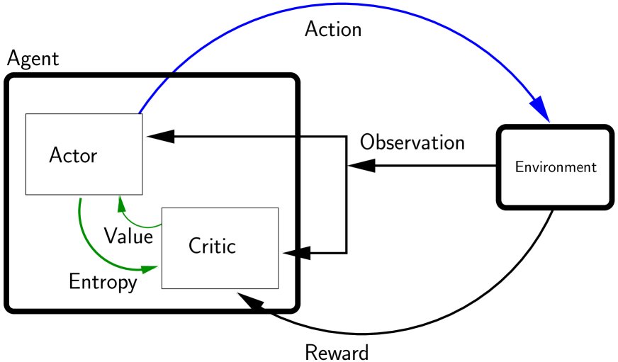
Figure 3: A reinforcement learning agent composed of an actor and a critic.

3.3.1 DDPG (Deep Deterministic Policy Gradient)

DDPG is an off-policy actor-critic algorithm for continuous action spaces.

Actor: Implements a deterministic policy network $\pi_\phi(s)$.
Critic: Implements a Q network $Q_\theta(s,a)$. It also uses target networks ($\pi_{\phi’}(s)$ and $Q_{\theta’}(s,a)$) to stabilize training.
Critic update: Updated by minimizing a loss function similar to DQN:

\[J(\theta) = \ \mid r(s,a) + \gamma Q_{\theta'} \left( s', \pi_{\phi'}(s') \right) - Q_{\theta}(s,a) \ \mid ^{2}\]

Actor update: Updated by maximizing the Q value given by the critic, i.e., minimizing the loss function:

\[J(\phi) = -Q_{\theta}\left(s, \pi_{\phi}(s)\right)\]

The target network parameters are softly updated through Polyak averaging, meaning they slowly track the parameters of the main network.

3.3.2 TD3 (Twin Delayed DDPG)

TD3 is an improved version of DDPG, designed to address its Q-value overestimation and training instability issues. It mainly includes three key techniques:

Twin Critics: Uses two independent Q networks ($Q_{\theta_1}, Q_{\theta_2}$) and takes the smaller of the two when computing the target Q value. This effectively suppresses Q-value overestimation.

\[J(\theta_i) = \ \mid r(s,a) + \gamma \underset{j=[1,2]}{\mathrm{min}} Q_{\theta'_{j}}\left(s',a'\right) - Q_{\theta_i}(s,a)\ \mid ^{2}\]

Delayed Policy Updates: The actor (policy network) is updated less frequently than the critic (Q network), for example, the actor is updated once for every two critic updates. This allows the Q-value estimates to become more stable before guiding policy improvement.
Target Policy Smoothing: When computing the target Q value, a small amount of noise is added to the action output by the target actor network and then clipped, making the Q function less sensitive to small changes in the action and thereby smoothing the value function estimate.

3.3.3 SAC (Soft Actor-Critic)

SAC is an off-policy actor-critic algorithm based on the maximum entropy reinforcement learning framework. Unlike DDPG/TD3, SAC uses a stochastic policy $\pi(a \mid s)$.

Core idea: The objective of SAC is not only to maximize cumulative reward, but also to maximize the policy’s entropy. Entropy measures the randomness of the policy and encourages the agent to explore more broadly.
Policy: The actor network $\pi_\phi(a \mid s)$ outputs a probability distribution (such as a Gaussian distribution), from which actions are sampled.
Critic update: Similar to TD3, SAC also uses two Q networks to suppress overestimation. Its loss function adds a term related to policy entropy on top of TD3 (proportional to $-\log\pi_\phi(a \mid s)$), so that while the reward is higher, the policy is also more stochastic.

\[J(\theta_i) = \ \mid r(s,a) + \gamma \left( \underset{j=[1,2]}{\mathrm{min}} Q_{\theta'_{j}}(s',a') - \alpha \log\pi_\phi(a' \mid s') \right) - Q_{\theta_i}(s,a)\ \mid ^2\]

Here, $\alpha$ is a temperature coefficient that balances reward and entropy, which can be manually tuned or learned automatically. This intrinsic exploration mechanism often gives SAC excellent performance in terms of sample efficiency and robustness.